Deep Q Networks (DQN)
Link to the paper: Mnih et al. (Google DeepMind) (2013), and Mnih et al. (DeepMind) (2015)
Introduction
This paper arguably launched the field of deep reinforcement learning. The paper was published in 2013, only a year after AlexNet brought convolutional neural networks (CNN) into the public eye after a show-stopping error rate of 15.4% on the ImageNet ILSVRC. The DQN paper was the first to successfully bring the powerful perception of CNNs to the reinforcement learning problem.
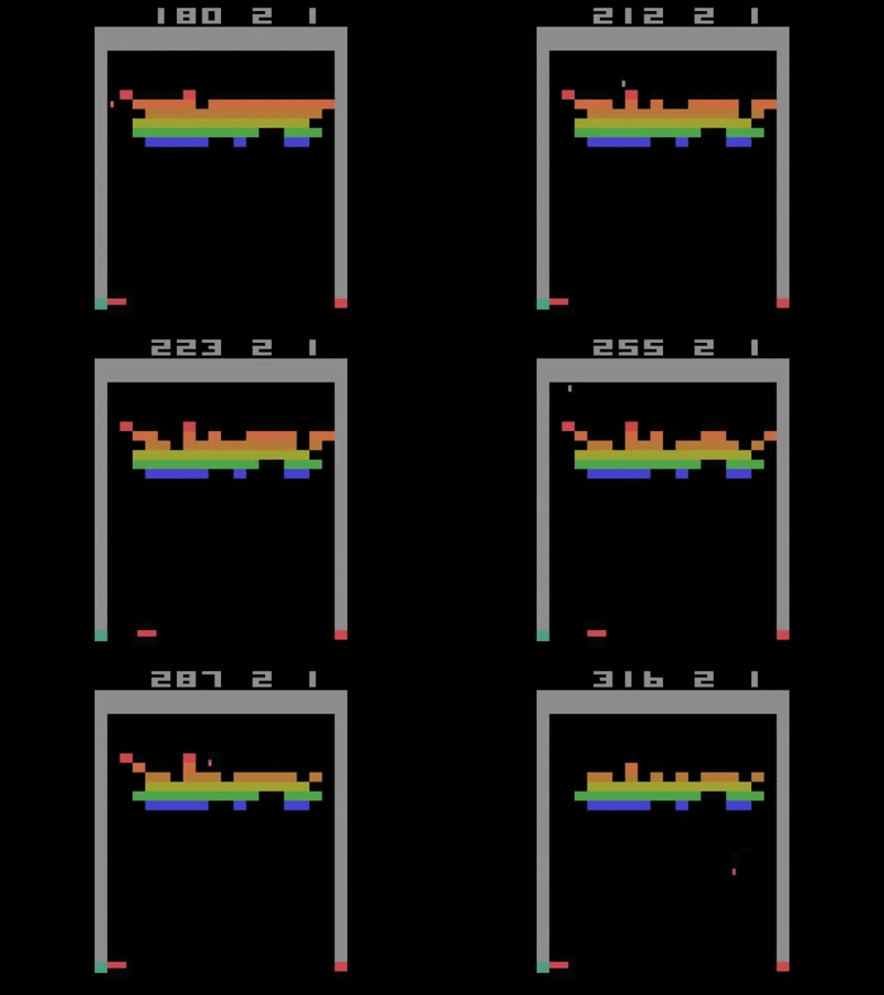
This architecture was trained separately on seven games from Atari 2600 from the Arcade Learning Environment. On six of the games, it surpassed all previous approaches, and on three of them, it beat human experts. Two years later, when the DQN article was featured in the journal Nature, it achieved human performance on 49 separate games. The optimal policy was even learned on Breakout, for example—focusing fire on the side, and getting the ball stuck in the top of the screen.

The DQN showing optimal strategy on Breakout—moving the ball into the top zone.
Since then, a lot of progress has been made, and DQN is no longer the architecture of choice for new problems. However, for the time, it was revolutionary. Google proceeded to buy DeepMind Technologies for more than $500M USD. Let's start by talking about the intuition behind DQN.
Basic idea
Rather than finding a policy directly, we can approximate the optimal action-value function, . This function maps state-action pairs to their expected discounted return. Then, finding the optimal policy would be simple: . We just choose the action at every step that greedily maximizes our action-value function.
The goal of the DQN architecture is to train a network to approximate the function.
First, we will introduce the objective function and network architecture. Then, we will discuss some of the pitfalls of the training procedure (hint: it's unstable). There are many add-ons to the DQN architecture which makes it perform much better, and we will discuss those in subsequent articles.
The loss function
First, we can write the Bellman optimality equation for :
However, this Bellman optimality equation only holds when has converged to the optimal policy . Otherwise, there will be some difference between and . Note that because is a Q-greedy policy. This difference known as the temporal difference error :
Our goal is to minimize this quantity. Our loss will be defined as the squared temporal difference error, similar to a mean squared error metric.
We will use this gradient to update the weights of our -network, because it will drive our network weights to producing the optimal -function and hence the optimal policy .
The neural network architecture
Since the function is approximating a Q function, we require that the input to the neural network be the state variables, and the output be the predicted Q-values.
Preprocessing
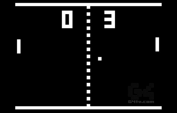
For most games, only providing images to the network isn't enough. Consider a simple game of Pong. A single frame is not enough information to determine the optimal action. Even though we know the ball position, we don't know the velocity.

Is the ball moving left or right?
There are many ways of getting around this:
- Use a recurrent neural network architecture, which summarizes the previous frames into a latent space vector;
- Use difference frames—subtract adjacent frames and feed that as input to the model;
- Stack frames together to see several previous frames in the current observation.
The DQN paper uses the latter technique—the last four frames are stacked together. In addition, there is some cropping work done to ensure small, square, grayscale images, although this is not strictly necessary. This produces (84 x 84 x 4) observation frames.
Architecture
Due to the visual structure of the Atari Learning Environment games, the authors of the DQN paper chose to use a convolutional neural network (CNN). The CNN has the following layers:
| Layer type | Details | Activation |
|---|---|---|
| Input | (84 x 84 x 4) input produced by preprocessing | |
| Convolution | 16 (8 x 8) filters, stride 4 | ReLU |
| Convolution | 32 (4 x 4) filters, stride 2 | ReLU |
| Dense | 256 hidden units | ReLU |
| Dense (output) | One output unit per action, representing the predicted Q-value | Linear |
This model was trained with the optimizer RMSProp.